Main Content

anovan

N-way analysis of variance

Description

example

p = anovan(y,group) returns a vector of p-values, one per term, for multiway (n-way) analysis of variance (ANOVA) for testing the effects of multiple factors on the mean of the vector y.

anovan also displays a figure showing the standard ANOVA table.

example

p = anovan(y,group,Name,Value) returns a vector of p-values for multiway (n-way) ANOVA using additional options specified by one or more Name,Value pair arguments.

For example, you can specify which predictor variable is continuous, if any, or the type of sum of squares to use.

[p,tbl] = anovan(___) returns the ANOVA table (including factor labels) in cell array tbl for any of the input arguments specified in the previous syntaxes. Copy a text version of the ANOVA table to the clipboard by using the Copy Text item on the Edit menu.

example

[p,tbl,stats] = anovan(___) returns a stats structure that you can use to perform a multiple comparison test, which enables you to determine which pairs of group means are significantly different. You can perform such a test using the multcompare function by providing the stats structure as input.

[p,tbl,stats,terms] = anovan(___) returns the main and interaction terms used in the ANOVA computations in terms.

Examples

collapse all

Load the sample data.

y = [52.7 57.5 45.9 44.5 53.0 57.0 45.9 44.0]';
g1 = [1 2 1 2 1 2 1 2]; 
g2 = {'hi';'hi';'lo';'lo';'hi';'hi';'lo';'lo'}; 
g3 = {'may';'may';'may';'may';'june';'june';'june';'june'};

y is the response vector and g1, g2, and g3 are the grouping variables (factors). Each factor has two levels, and every observation in y is identified by a combination of factor levels. For example, observation y(1) is associated with level 1 of factor g1, level 'hi' of factor g2, and level 'may' of factor g3. Similarly, observation y(6) is associated with level 2 of factor g1, level 'hi' of factor g2, and level 'june' of factor g3.

Test if the response is the same for all factor levels.

p = anovan(y,{g1,g2,g3})

Figure N-Way ANOVA contains objects of type uicontrol.

p = 3×1

    0.4174
    0.0028
    0.9140

In the ANOVA table, X1, X2, and X3 correspond to the factors g1, g2, and g3, respectively. The p-value 0.4174 indicates that the mean responses for levels 1 and 2 of the factor g1 are not significantly different. Similarly, the p-value 0.914 indicates that the mean responses for levels 'may' and 'june', of the factor g3 are not significantly different. However, the p-value 0.0028 is small enough to conclude that the mean responses are significantly different for the two levels, 'hi' and 'lo' of the factor g2. By default, anovan computes p-values just for the three main effects.

Test the two-factor interactions. This time specify the variable names.

p = anovan(y,{g1 g2 g3},'model','interaction','varnames',{'g1','g2','g3'})

Figure N-Way ANOVA contains objects of type uicontrol.

p = 6×1

    0.0347
    0.0048
    0.2578
    0.0158
    0.1444
    0.5000

The interaction terms are represented by g1*g2, g1*g3, and g2*g3 in the ANOVA table. The first three entries of p are the p-values for the main effects. The last three entries are the p-values for the two-way interactions. The p-value of 0.0158 indicates that the interaction between g1 and g2 is significant. The p-values of 0.1444 and 0.5 indicate that the corresponding interactions are not significant.

Load the sample data.

load carbig

The data has measurements on 406 cars. The variable org shows where the cars were made and when shows when in the year the cars were manufactured.

Study how the mileage depends on when and where the cars were made. Also include the two-way interactions in the model.

p = anovan(MPG,{org when},'model',2,'varnames',{'origin','mfg date'})

Figure N-Way ANOVA contains objects of type uicontrol.

p = 3×1

    0.0000
    0.0000
    0.3059

The 'model',2 name-value pair argument represents the two-way interactions. The p-value for the interaction term, 0.3059, is not small, indicating little evidence that the effect of the time of manufacture (mfg date) depends on where the car was made (origin). The main effects of origin and manufacturing date, however, are significant, both p-values are 0.

Load the sample data.

y = [52.7 57.5 45.9 44.5 53.0 57.0 45.9 44.0]';
g1 = [1 2 1 2 1 2 1 2];
g2 = ["hi" "hi" "lo" "lo" "hi" "hi" "lo" "lo"];
g3 = ["may" "may" "may" "may" "june" "june" "june" "june"];

y is the response vector and g1, g2, and g3 are the grouping variables (factors). Each factor has two levels, and every observation in y is identified by a combination of factor levels. For example, observation y(1) is associated with level 1 of factor g1, level hi of factor g2, and level may of factor g3. Similarly, observation y(6) is associated with level 2 of factor g1, level hi of factor g2, and level june of factor g3.

Test if the response is the same for all factor levels. Also compute the statistics required for multiple comparison tests.

[~,~,stats] = anovan(y,{g1 g2 g3},"Model","interaction", ...
    "Varnames",["g1","g2","g3"]);

Figure N-Way ANOVA contains objects of type uicontrol.

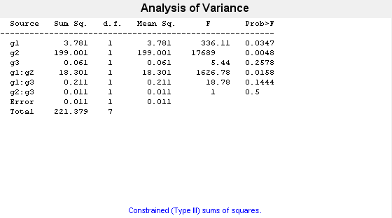
The p-value of 0.2578 indicates that the mean responses for levels may and june of factor g3 are not significantly different. The p-value of 0.0347 indicates that the mean responses for levels 1 and 2 of factor g1 are significantly different. Similarly, the p-value of 0.0048 indicates that the mean responses for levels hi and lo of factor g2 are significantly different.

Perform a multiple comparison test to find out which groups of factors g1 and g2 are significantly different.

[results,~,~,gnames] = multcompare(stats,"Dimension",[1 2]);

Figure Multiple comparison of population marginal means contains an axes object. The axes object with title Click on the group you want to test, xlabel 3 groups have population marginal means significantly different from g1=1,g2=hi contains 9 objects of type line. One or more of the lines displays its values using only markers

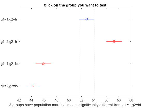
You can test the other groups by clicking on the corresponding comparison interval for the group. The bar you click on turns to blue. The bars for the groups that are significantly different are red. The bars for the groups that are not significantly different are gray. For example, if you click on the comparison interval for the combination of level 1 of g1 and level lo of g2, the comparison interval for the combination of level 2 of g1 and level lo of g2 overlaps, and is therefore gray. Conversely, the other comparison intervals are red, indicating significant difference.

Display the multiple comparison results and the corresponding group names in a table.

tbl = array2table(results,"VariableNames", ...
    ["Group A","Group B","Lower Limit","A-B","Upper Limit","P-value"]);
tbl.("Group A")=gnames(tbl.("Group A"));
tbl.("Group B")=gnames(tbl.("Group B"))
tbl=6×6 table
       Group A           Group B        Lower Limit     A-B     Upper Limit     P-value 
    ______________    ______________    ___________    _____    ___________    _________

    {'g1=1,g2=hi'}    {'g1=2,g2=hi'}      -6.8604       -4.4      -1.9396       0.027249
    {'g1=1,g2=hi'}    {'g1=1,g2=lo'}       4.4896       6.95       9.4104       0.016983
    {'g1=1,g2=hi'}    {'g1=2,g2=lo'}       6.1396        8.6        11.06       0.013586
    {'g1=2,g2=hi'}    {'g1=1,g2=lo'}       8.8896      11.35        13.81       0.010114
    {'g1=2,g2=hi'}    {'g1=2,g2=lo'}        10.54         13        15.46      0.0087375
    {'g1=1,g2=lo'}    {'g1=2,g2=lo'}      -0.8104       1.65       4.1104        0.07375

The multcompare function compares the combinations of groups (levels) of the two grouping variables, g1 and g2. For example, the first row of the matrix shows that the combination of level 1 of g1 and level hi of g2 has the same mean response values as the combination of level 2 of g1 and level hi of g2. The p-value corresponding to this test is 0.0272, which indicates that the mean responses are significantly different. You can also see this result in the figure. The blue bar shows the comparison interval for the mean response for the combination of level 1 of g1 and level hi of g2. The red bars are the comparison intervals for the mean response for other group combinations. None of the red bars overlap with the blue bar, which means the mean response for the combination of level 1 of g1 and level hi of g2 is significantly different from the mean response for other group combinations.

Input Arguments

collapse all

Sample data, specified as a numeric vector.

Data Types: single | double

Grouping variables, i.e. the factors and factor levels of the observations in y, specified as a cell array. Each of the cells in group contains a list of factor levels identifying the observations in y with respect to one of the factors. The list within each cell can be a categorical array, numeric vector, character matrix, string array, or single-column cell array of character vectors, and must have the same number of elements as y.

y=[y1,y2,y3,y4,y5,,yN]g1={'A','A','C','B','B',,'D'}g2=[12131,2]g3={'hi','mid','low','mid','hi',,'low'}

By default, anovan treats all grouping variables as fixed effects.

For example, in a study you want to investigate the effects of gender, school, and the education method on the academic success of elementary school students, then you can specify the grouping variables as follows.

Example: {'Gender','School','Method'}

Data Types: cell

Name-Value Arguments

Specify optional pairs of arguments as Name1=Value1,...,NameN=ValueN, where Name is the argument name and Value is the corresponding value. Name-value arguments must appear after other arguments, but the order of the pairs does not matter.

Before R2021a, use commas to separate each name and value, and enclose Name in quotes.

Example: 'alpha',0.01,'model','interaction','sstype',2 specifies anovan to compute the 99% confidence bounds and p-values for the main effects and two-way interactions using type II sum of squares.

Significance level for confidence bounds, specified as the comma-separated pair consisting of'alpha' and a scalar value in the range 0 to 1. For a value α, the confidence level is 100*(1–α)%.

Example: 'alpha',0.01 corresponds to 99% confidence intervals

Data Types: single | double

Indicator for continuous predictors, representing which grouping variables should be treated as continuous predictors rather than as categorical predictors, specified as the comma-separated pair consisting of 'continuous' and a vector of indices.

For example, if there are three grouping variables and second one is continuous, then you can specify as follows.

Example: 'continuous',[2]

Data Types: single | double

Indicator to display ANOVA table, specified as the comma-separated pair consisting of 'display' and 'on' or 'off'. When 'display' is 'off', anovan only returns the output arguments, and does not display the standard ANOVA table as a figure.

Example: 'display','off'

Type of the model, specified as the comma-separated pair consisting of 'model' and one of the following:

  • 'linear' — The default 'linear' model computes only the p-values for the null hypotheses on the N main effects.

  • 'interaction' — The 'interaction' model computes the p-values for null hypotheses on the N main effects and the (N2) two-factor interactions.

  • 'full' — The 'full' model computes the p-values for null hypotheses on the N main effects and interactions at all levels.

  • An integer — For an integer value of k, (kN) for model type, anovan computes all interaction levels through the kth level. For example, the value 3 means main effects plus two- and three-factor interactions. The values k = 1 and k = 2 are equivalent to the 'linear' and 'interaction' specifications, respectively. The value k = N is equivalent to the 'full' specification.

  • Terms matrix — A matrix of term definitions having the same form as the input to the x2fx function. All entries must be 0 or 1 (no higher powers).

    For more precise control over the main and interaction terms that anovan computes, you can specify a matrix containing one row for each main or interaction term to include in the ANOVA model. Each row defines one term using a vector of N zeros and ones. The table below illustrates the coding for a 3-factor ANOVA for factors A, B, and C.

    Matrix RowANOVA Term

    [1 0 0]

    Main term A

    [0 1 0]

    Main term B

    [0 0 1]

    Main term C

    [1 1 0]

    Interaction term AB

    [1 0 1]

    Interaction term AC

    [0 1 1]

    Interaction term BC

    [1 1 1]

    Interaction term ABC

    For example, if there are three factors A, B, and C, and 'model',[0 1 0;0 0 1;0 1 1], then anovan tests for the main effects B and C, and the interaction effect BC, respectively.

    A simple way to generate the terms matrix is to modify the terms output, which codes the terms in the current model using the format described above. If anovan returns [0 1 0;0 0 1;0 1 1] for terms, for example, and there is no significant interaction BC, then you can recompute ANOVA on just the main effects B and C by specifying [0 1 0;0 0 1] for model.

Example: 'model',[0 1 0;0 0 1;0 1 1]

Example: 'model','interaction'

Data Types: char | string | single | double

Nesting relationships among the grouping variables, specified as the comma-separated pair consisting of 'nested' and a matrix M of 0’s and 1’s, i.e.M(i,j) = 1 if variable i is nested in variable j.

You cannot specify nesting in a continuous variable.

For example, if there are two grouping variables District and School, where School is nested in District, then you can express this relationship as follows.

Example: 'nested',[0 0;1 0]

Data Types: single | double

Indicator for random variables, representing which grouping variables are random, specified as the comma-separated pair consisting of 'random' and a vector of indices. By default, anovan treats all grouping variables as fixed.

anovan treats an interaction term as random if any of the variables in the interaction term is random.

Example: 'random',[3]

Data Types: single | double

Type of sum squares, specified as the comma-separated pair consisting of 'sstype' and the following:

  • 1 — Type I sum of squares. The reduction in residual sum of squares obtained by adding that term to a fit that already includes the terms listed before it.

  • 2 — Type II sum of squares. The reduction in residual sum of squares obtained by adding that term to a model consisting of all other terms that do not contain the term in question.

  • 3 — Type III sum of squares. The reduction in residual sum of squares obtained by adding that term to a model containing all other terms, but with their effects constrained to obey the usual “sigma restrictions” that make models estimable.

  • 'h' — Hierarchical model. Similar to type 2, but with continuous as well as categorical factors used to determine the hierarchy of terms.

The sum of squares for any term is determined by comparing two models. For a model containing main effects but no interactions, the value of sstype influences the computations on unbalanced data only.

Suppose you are fitting a model with two factors and their interaction, and the terms appear in the order A, B, AB. Let R(·) represent the residual sum of squares for the model. So, R(A, B, AB) is the residual sum of squares fitting the whole model, R(A) is the residual sum of squares fitting the main effect of A only, and R(1) is the residual sum of squares fitting the mean only. The three sum of squares types are as follows:

TermType 1 Sum of SquaresType 2 Sum of SquaresType 3 Sum of Squares

A

R(1) – R(A)

R(B) – R(A, B)

R(B, AB) – R(A, B, AB)

B

R(A) – R(A, B)

R(A) – R(A, B)

R(A, AB) – R(A, B, AB)

AB

R(A, B) – R(A, B, AB)

R(A, B) – R(A, B, AB)

R(A, B) – R(A, B, AB)

The models for Type 3 sum of squares have sigma restrictions imposed. This means, for example, that in fitting R(B, AB), the array of AB effects is constrained to sum to 0 over A for each value of B, and over B for each value of A.

Example: 'sstype','h'

Data Types: single | double | char | string

Names of grouping variables, specified as the comma-separating pair consisting of 'varnames' and a character matrix, a string array, or a cell array of character vectors.

Example: 'varnames',{'Gender','City'}

Data Types: char | string | cell

Output Arguments

collapse all

p-values, returned as a vector.

Output vector p contains p-values for the null hypotheses on the N main effects and any interaction terms specified. Element p(1) contains the p-value for the null hypotheses that samples at all levels of factor A are drawn from the same population; element p(2) contains the p-value for the null hypotheses that samples at all levels of factor B are drawn from the same population; and so on.

For example, if there are three factors A, B, and C, and 'model',[0 1 0;0 0 1;0 1 1], then the output vector p contains the p-values for the null hypotheses on the main effects B and C and the interaction effect BC, respectively.

A sufficiently small p-value corresponding to a factor suggests that at least one group mean is significantly different from the other group means; that is, there is a main effect due to that factor. It is common to declare a result significant if the p-value is less than 0.05 or 0.01.

ANOVA table, returned as a cell array. The ANOVA table has seven columns:

Column nameDefinition
sourceSource of the variability.
SSSum of squares due to each source.
dfDegrees of freedom associated with each source.
MSMean squares for each source, which is the ratio SS/df.
Singular?Indication of whether the term is singular.
FF-statistic, which is the ratio of the mean squares.
Prob>FThe p-values, which is the probability that the F-statistic can take a value larger than a computed test-statistic value. anovan derives these probabilities from the cdf of F-distribution.

The ANOVA table also contains the following columns if at least one of the grouping variables is specified as random using the name-value pair argument random:

Column nameDefinition
TypeType of each source; 'fixed' for a fixed effect or 'random' for a random effect.
Expected MSText representation of the expected value for the mean square. Q(source) represents a quadratic function of source and V(source) represents the variance of source.
MS denomDenominator of the F-statistic.
d.f. denomDegrees of freedom for the denominator of the F-statistic.
Denom. defn.Text representation of the denominator of the F-statistic. MS(source) represents the mean square of source.
Var. est.Variance component estimate.
Var. lower bndLower bound of the 95% confidence interval for the variance component estimate.
Var. upper bndUpper bound of the 95% confidence interval for the variance component estimate.

Statistics to use in a multiple comparison test using the multcompare function, returned as a structure.

anovan evaluates the hypothesis that the different groups (levels) of a factor (or more generally, a term) have the same effect, against the alternative that they do not all have the same effect. Sometimes it is preferable to perform a test to determine which pairs of levels are significantly different, and which are not. Use the multcompare function to perform such tests by supplying the stats structure as input.

The stats structure contains the fields listed below, in addition to a number of other fields required for doing multiple comparisons using the multcompare function:

FieldDescription

coeffs

Estimated coefficients

coeffnames

Name of term for each coefficient

vars

Matrix of grouping variable values for each term

resid

Residuals from the fitted model

The stats structure also contains the following fields if at least one of the grouping variables is specified as random using the name-value pair argument random:

FieldDescription

ems

Expected mean squares

denom

Denominator definition

rtnames

Names of random terms

varest

Variance component estimates (one per random term)

varci

Confidence intervals for variance components

Main and interaction terms, returned as a matrix. The terms are encoded in the output matrix terms using the same format described above for input model. When you specify model itself in this format, the matrix returned in terms is identical.

Alternative Functionality

Instead of using anovan, you can create an anova object by using the anova function. The anova function provides these advantages:

  • The anova function allows you to specify the ANOVA model type, sum of squares type, and factors to treat as categorical. anova also supports table predictor and response input arguments.

  • In addition to the outputs returned by anovan, the properties of the anova object contain the following:

    • ANOVA model formula

    • Fitted ANOVA model coefficients

    • Residuals

    • Factors and response data

  • The anova object functions allow you to conduct further analysis after fitting the anova object. For example, you can create an interactive plot of multiple comparisons of means for the ANOVA, get the mean response estimates for each value of a factor, and calculate the variance component estimates.

References

[1] Dunn, O.J., and V.A. Clark. Applied Statistics: Analysis of Variance and Regression. New York: Wiley, 1974.

[2] Goodnight, J.H., and F.M. Speed. Computing Expected Mean Squares. Cary, NC: SAS Institute, 1978.

[3] Seber, G. A. F., and A. J. Lee. Linear Regression Analysis. 2nd ed. Hoboken, NJ: Wiley-Interscience, 2003.

Version History

Introduced before R2006a