Solving Large-Scale Optimization Problems with MATLAB: A Hydroelectric Flow Example
By Seth DeLand, MathWorks
Setting up and solving a large optimization problem for portfolio optimization, constrained data fitting, parameter estimation, or other applications can be a challenging task. As a result, it is common to first set up and solve a smaller, simpler version of the problem and then scale up to the large-scale problem. Working with a smaller version reduces the time that it takes to identify key relationships in the model, makes the model easier to debug, and enables you to identify an efficient solution that can be used for the large-scale problem.
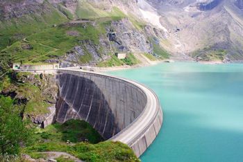
This article describes three techniques for finding a control strategy for optimal operation of a hydroelectric dam (Figure 1): using a nonlinear optimization algorithm, a nonlinear optimization algorithm with derivative functions, and quadratic programming.
Working with MATLAB®, Optimization Toolbox™ and Symbolic Math Toolbox™, we will start by solving a smaller version of the problem and then scale up to the large-scale problem once we have found an appropriate solution method.
The MATLAB code used in this example is available for download.
Optimization Goal
Our hydroelectric power plant model includes the inlet flow into the reservoir from the river and the storage level of the reservoir (Figure 2).
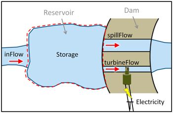
Water can leave the reservoir either through the spillway or via the turbine. Water that leaves through the turbine is used to generate electricity. We can sell this electricity at prices that are determined by various market factors. We control the rates at which water flows through the spillway and the turbine. Our goal is to find values for these rates that will maximize revenue over the long term.
The best values for the hydroelectric flow rates are found over several days at hourly intervals. As a result, we need to find the flow values at each hour, which means that the size of the problem will increase the longer we run the optimization.
Defining System Interactions Using Symbolic Variables
We use the following equations to describe the interactions in this system. The first is the empirical equation for the turbine, and relates the electricity produced to the turbine flow and reservoir level. The second gives the reservoir storage level as a function of the flow into and out of the reservoir.
Electricity(t) = TurbineFlow(t-1)*[½ k1(Storage(t) + Storage(t-1)) + k2]
Storage(t) = Storage(t-1) + ∆t * [inFlow(t-1) - spillFlow(t-1) - turbineFlow(t-1)]
The amount of electricity produced is a function of the amount of water flowing to the turbine and the storage level in the reservoir. This means that the higher the water level in the reservoir, the more power will be produced for a given turbine flow.
Certain constraints need to be taken into consideration. Both the reservoir level and downstream flow rates must remain within specified ranges. The maximum level of flow that the turbine can handle is set, but the spillway level is unrestricted. Additionally, the reservoir level at the end of the simulation must be the same as the level at the start of the simulation. The power plant will continue to operate beyond the period for which we are optimizing, so we need to prevent the solver from finding a solution that empties the reservoir.
All the constraints for this problem are linear, meaning they can be expressed in matrix notation. Our objective, however, is nonlinear, making it challenging to express. We begin by formulating the objective function using symbolic variables.
X = sym('x',[2*N,1]);   % turbine flow and spill flow
F = sym('F',[N,1]);     % flow into the reservoir
P = sym('P',[N,1]);     % price
s0 = sym('s0');         % initial storage
c = sym({'c1','c2','c3','c4'}.','r');   % constants

% Total out flow equation
TotFlow = X(1:N)+X(N+1:end); % turbine flow + spill flow
% Storage Equations
S = cell(N,1);
S{1} = s0 + c(1)*(F(1)-TotFlow(1));
for ii = 2:N
S{ii} = S{ii-1} + c(1)*(F(ii)-TotFlow(ii));
end
% K factor equation
k = c(2)*([s0; S(1:end-1)]+ S)/2+c(3);
% Megawatt-hours equation
MWh = k.*X(1:N)/c(4);
% Revenue equation
R = P.*MWh;
% Total Revenue (Minus sign changes from maximization to minimization)
totR = -sum(R);
We convert this symbolic representation of our objective function into a MATLAB function using the matlabfunction command.
Nonlinear Optimization
We can now solve this problem using fmincon, a general nonlinear optimization solver.
% Perform substitutions so that X is the only remaining variable
totR = subs(totR,[c;s0;P;F],[C';stor0;price;inFlow]);
% Generate a MATLAB file from the equation
matlabFunction(totR,'vars',{X},'file','objFcn');
%% 5 - Optimize with FMINCON
options = optimset('MaxFunEvals',Inf,'MaxIter',5000,...
'Algorithm','interior-point');
[x1, fval1] = fmincon(@objFcn,x0,A,b,Aeq,beq,LB,UB,[],options);
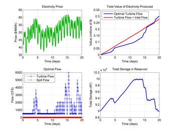
Figure 3 shows the optimization results, together with the electricity price data that was used.

Figure 3. Optimal turbine and spill flows for given electricity prices.
We see that the optimal operation sends no water to the spillway, and sends more water to the turbine when electricity prices rise.
Speeding Up Calculations with Derivative Functions
The fmincon solver took 21.4 seconds to find the solution. Much of this time was spent approximating the gradient of the objective function using finite differences. One way to speed up this optimization problem is to supply the solver with functions that analytically calculate its gradient and Hessian. Because we defined our objective function using symbolic math, we can use the gradient and hessian functions from Symbolic Math Toolbox to calculate these functions automatically.
gradObj = gradient(totR,X); % Gradient
matlabFunction(gradObj,'vars',{X},'file','grad');
% Create a function that returns the objective value and gradient
ValAndGrad = @(x) deal(objFcn(x),grad(x));
hessObj = hessian(totR,X); % Hessian
matlabFunction(hessObj,'vars',{X},'file','Hess');
hfcn = @(x,lambda) Hess(x); % Function handle to hessian
% Optimize
options = optimset(options,'GradObj','on','Hessian','user-supplied',...
'HessFcn',hfcn);
[x2,fval2] = fmincon(ValAndGrad,x0,A,b,Aeq,beq,LB,UB,[],options);
This time, the problem was solved in 0.25 seconds. By specifying the gradient and the Hessian for this problem, we achieved an 85-fold speedup.
Quadratic Programming
A closer look at the Hessian matrix for this problem reveals that it is a constant: the values in the matrix are independent of the decision variables. This is a sign that the problem is quadratic, because its partial second derivatives are constant. As a result, we can use the quadprog solver in Optimization Toolbox, which was designed for large quadratic problems like this one. The constraint matrices will remain unchanged, since fmincon and quadprog use the same formulation for linear constraints.
We pass the objective function to quadprog in two parts: the Hessian matrix H and the vector of linear term coefficients f. The interior-point-convex algorithm for quadratic programming is the recommended algorithm for convex problems such as this one.
qpopts = optimset('Algorithm','interior-point-convex');
[x,fval] = quadprog(H,f',A,b,Aeq,beq,LB,UB,[],qpopts);
With the interior-point-convex algorithm, the optimal solution was found in 0.05 seconds. Because the interior-point-convex algorithm supports sparse matrices (H is 50% sparse, and A is 20% sparse), we can scale up and run the optimization over a larger data set.
Figure 4 shows that the optimal solution to the large-scale problem ran for YY days of data. Notice in the lower-right plot that the optimal solution found by quadprog stores water in the reservoir during the first part of the simulation, so that there is a large volume of water available for the 14th and 15th days, when electricity can be sold at higher prices.
We run the optimization problem for an increasing number of decision variables and compare the performance of the different solution methods. The results show that the interior-point-convex algorithm solved the 6400-variable problem (over 4 months of data) in less than half an hour (Table 1).
| Decision Variables |
fmincon(no gradient) |
fmincon(with gradient and Hessian) |
quadproginterior-point-convex |
|---|---|---|---|
| 100 | 16 s | 0.46 s | 0.04 s |
| 200 | 238 s | 1.24 s | 0.16 s |
| 400 | 965 s | 3.17 s | 0.77 s |
| 800 | 6083 s | 43 s | 5 s |
| 1600 | - | * | 30 s |
| 3200 | - | * | 190 s |
| 6400 | - | * | 1641 s |
Table 1. Comparison of optimization times for different solution methods.
*Gradient/Hessian generation took several hours.
Published 2012 - 92061v00